Conditional Formatting in Excel

 

Conditional Formatting

Learn how to add color & shapes to your data & reports to highlight key findings.

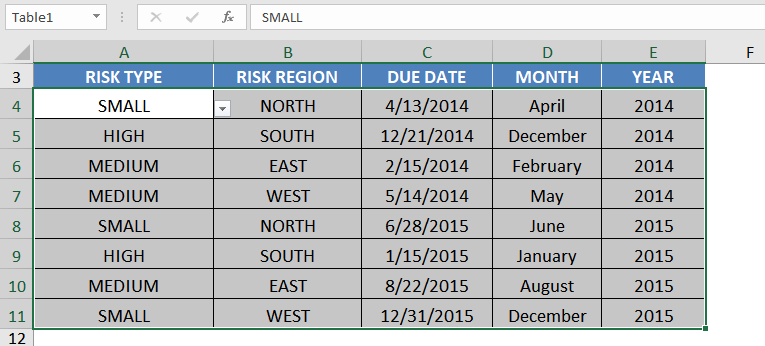
Conditionally Formatting a Drop Down List

We are now going to take this concept one level further and apply some conditional formatting to the drop down data validation list.

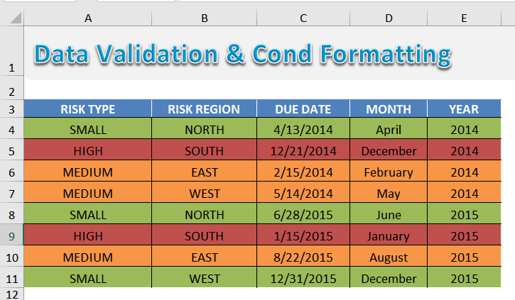
This is useful if you want to highlight when a job is completed, check off items from a list or to evaluate risk in a project just like I have done in below´s example.

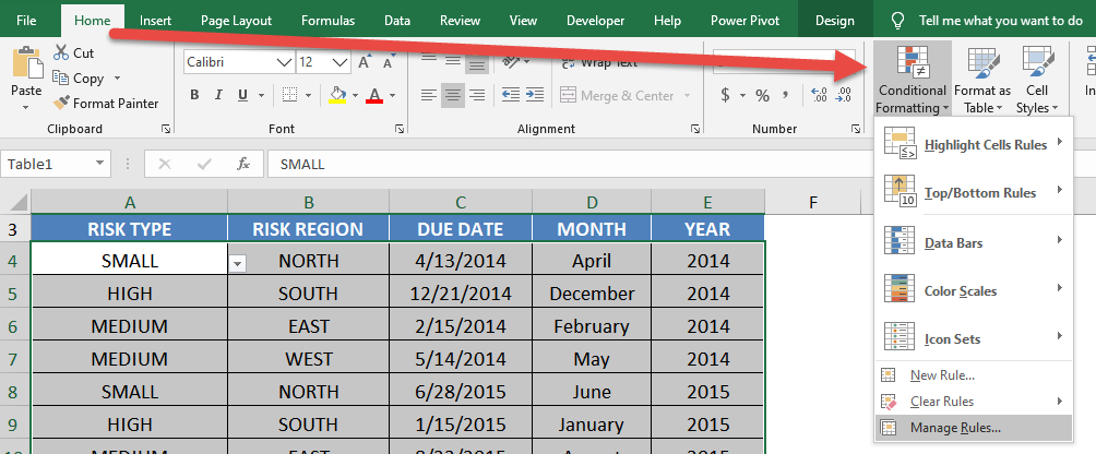
STEP 1: Select the range that you want to apply the conditional formatting to.

STEP 2: Go to Home > Styles > Conditional Formatting > Manage Rules

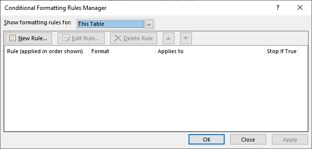
STEP 3: Select New Rule

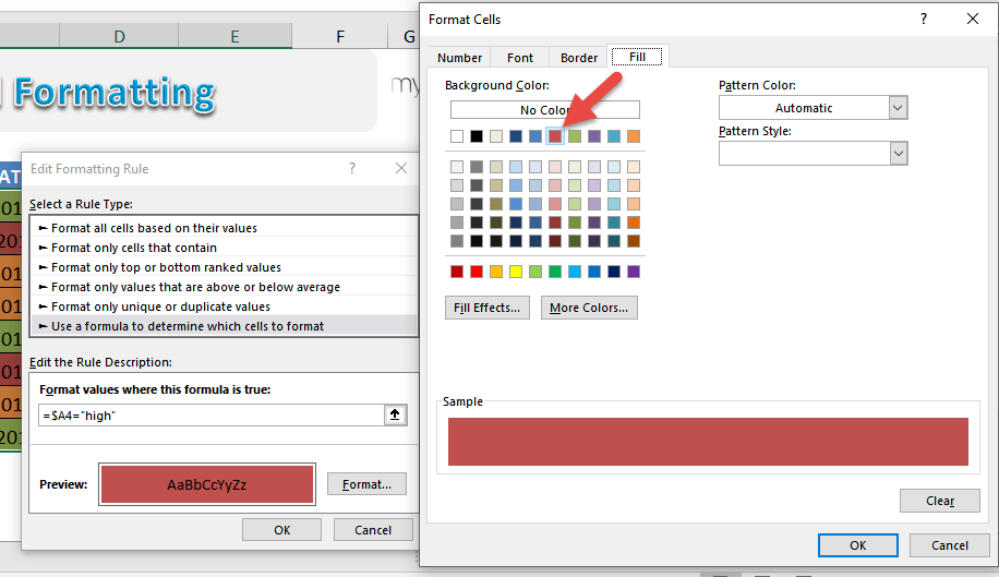
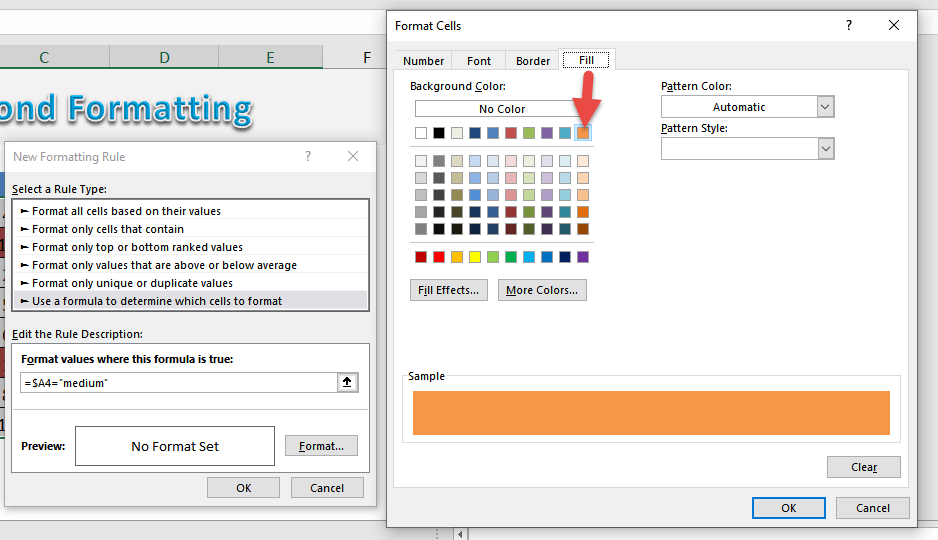
STEP 4: Create the new rule for High values:

Select Use a formula to determine which cells to format

Type in the Formula =$A4=”high” 

This formula will ensure only the column is absolute.

Go to Format > Fill then select a color of your choosing. Click OK.

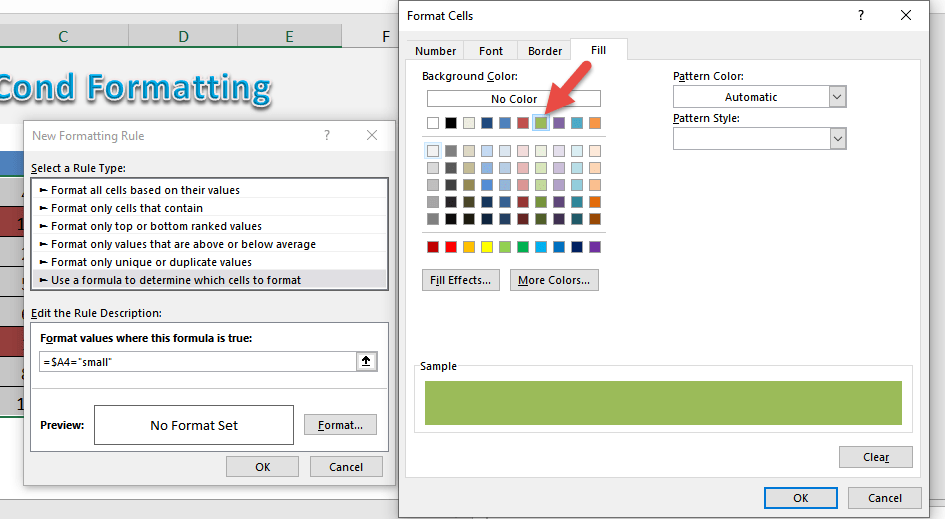
Repeat the same steps for medium values. Click New Rule.

Select Use a formula to determine which cells to format

Type in the Formula =$A4=”medium” 

This formula will ensure only the column is absolute.

Go to Format > Fill then select a color of your choosing. Click OK.

Repeat the same steps for low values. Click New Rule.

Select Use a formula to determine which cells to format

Type in the Formula =$A4=”low” 

This formula will ensure only the column is absolute.

Go to Format > Fill then select a color of your choosing. Click OK.

This is how our new set of rules will look like:

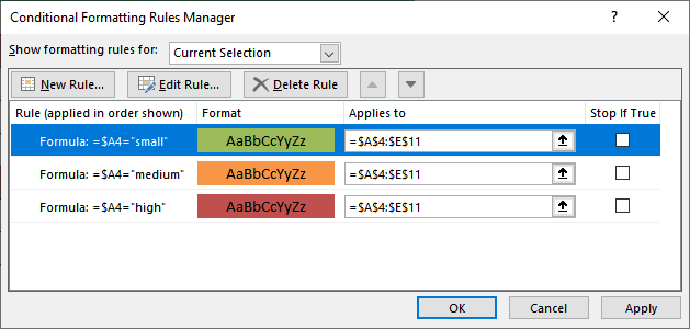
Now our table now has conditional formatting applied!

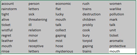
Find Duplicates Using Conditional Formatting

Normally when we have dirty data, we tend to get a lot of duplicates. But in Excel it is very easy to spot the duplicates for your data cleanup!

Here is our sample list of words, you can see it has a lot of duplicates:

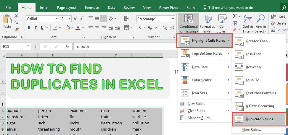
STEP 1:Select your list of words / data:

STEP 2: Go to Home > Conditional Formatting > Highlight Cells Rules > Duplicate Values

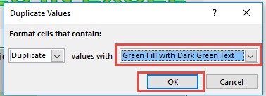
STEP 3: You can select the formatting that you want. For our example, we selected Green Fill with Dark Green Text.

Click OK.

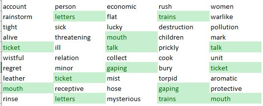
You will now see the magic happen, all of the duplicate values are now highlighted in your Excel worksheet!

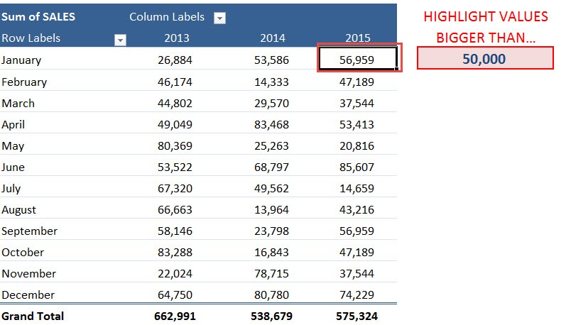
Conditionally Format a Cell’s Value

A great way to highlight values within your data set, Excel Table or Pivot Table is to use Conditional Formatting rules.

Formatting cells that contain a specific criteria, for example, greater than X or less than X, is a good way to visualize your results.

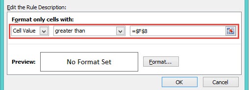
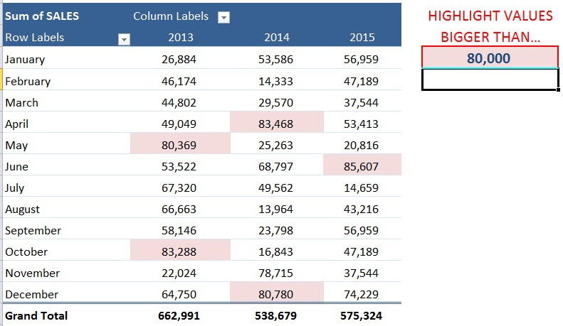
When your criteria references a cell, then you can make this conditional format interactive.  So as you manually change the referenced cell´s value, the conditional format gets updated and you can see the live results, as shown below….

STEP 1: Select a cell in your Pivot Table.

STEP 2: Go to Home > Conditional Formatting > New Rule

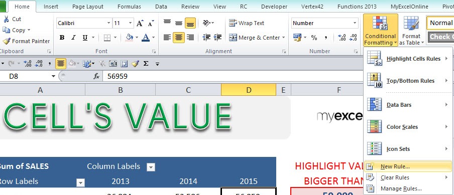
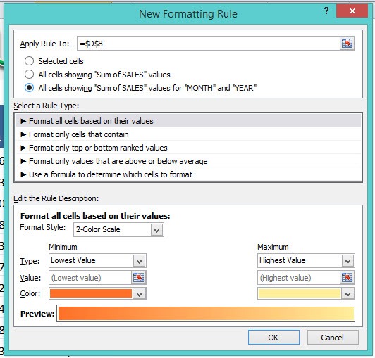
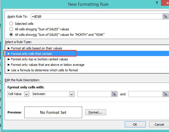
STEP 3: Set Apply Rule to the third option: All cells showing “Sum of SALES” values for “MONTH” and “YEAR”

STEP 4: Select a rule type: Format Only Cells That Contain

STEP 5: Edit the Rule Description. Go to Cell Value > Greater Than > Select The Cell

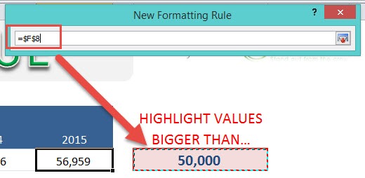
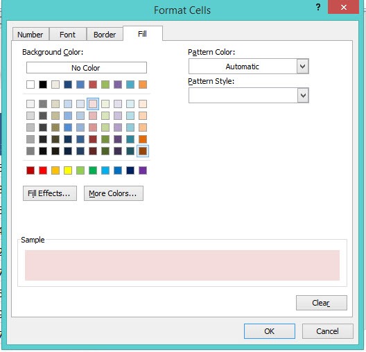
STEP 6: Select the cell format. Click Format and select a color. Click OK.

Try it out now! The highlight now happens dynamically when you update the value.