How to Use Windings Symbols in Excel

 

How to Use Windings Symbols in Excel

Wingdings is a symbolic font that a lot of us use for fun. I do that a lot too! But what if we wanted those cool symbols to be of good use in Excel?

Whenever I tried typing using the Wingdings font, I was not sure which symbol I would get!

I will show you how easy it is to pick a cool Wingdings Symbol and use it in your Excel worksheet!

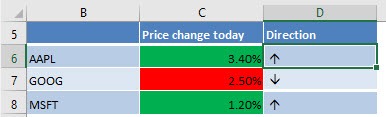
Here is a sample usage of a Wingdings symbol for stock prices:

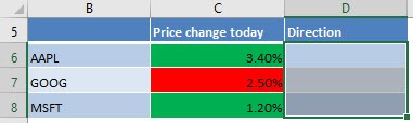
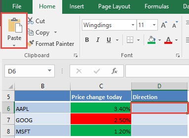
STEP 1: Select the cells that you want to place the symbols in:

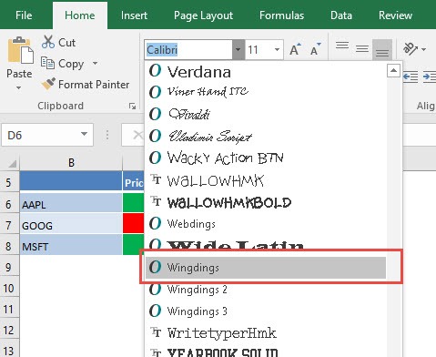
From the Font dropdown, select Wingdings:

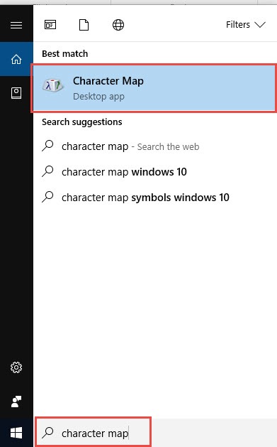
STEP 2: Now that our cells are able to accept Wingdings symbols, go to Windows Start (Windows 10) > Search Bar > Character Map

If you are have an older version of Windows, go to Start > All Programs > Accessories > System Tools > Character Map

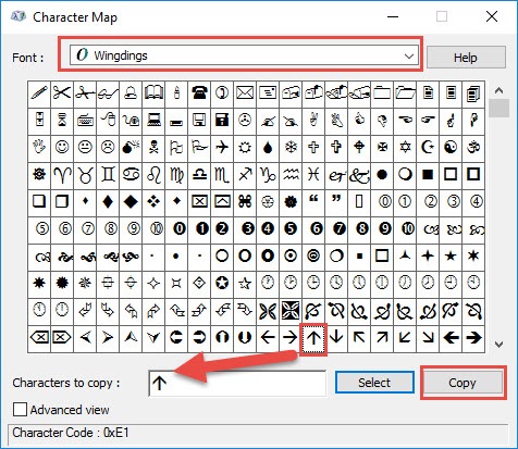
STEP 3: You will now see all the characters!  Ensure the Font is Wingdings.

Double click on the symbol you want to use. Click Copy.

STEP 4: Go to your Excel Spreadsheet and click Paste.

Do the rest for the other cells, and you have used Wingdings Symbols!

NOTE: Another way is to click in a blank cell and go to Insert > Symbol > Font: Windings > Insert > Close.

Evaluate Formulas Step By Step in Excel

This is one of the coolest tricks I have seen in Excel, as there are countless times wherein I had a hard time understand formulas. Especially long and complex ones!

Excel provides the way to evaluate your formula, and break it down step by step so that you can understand it!

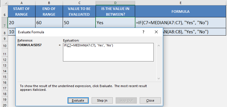
Let us take the formulas I’ve created below in the IS THE VALUE IN BETWEEN column . We will see how this formula is resolved in a series of steps:

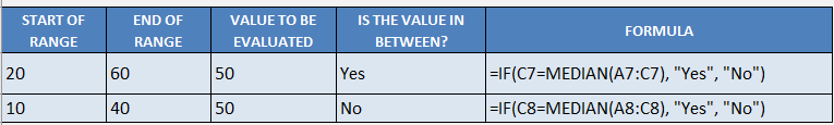
STEP 1: You can see our formula uses both the If formula and the Median formula. 

The goal of this formula is to evaluate if a value (VALUE TO BE EVALUATED) is in between the range (START OF RANGE to VALUE TO BE EVALUATED)

For example: Is 50 the median of the range 20; 60; 50?

=IF(C7=MEDIAN(A7:C7), “Yes”, “No”)

To start understanding our formula, highlight the formula, then go to Formulas > Evaluate Formula:

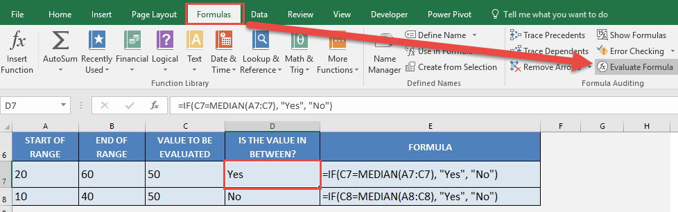
STEP 2: Our formula is now shown on screen, and the part that is underlined is the one to be evaluated first.  Click Evaluate.

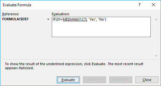
STEP 3: C7 has been evaluated to 50.  Click Evaluate.

STEP 4:  The median of the values from A7 to C7 (20, 60, 50) is evaluated as 50.  Click Evaluate.

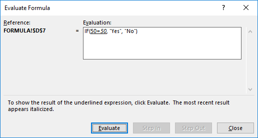
STEP 5:  Is 50 equal to 50?

Excel has evaluated it to TRUE.  Click Evaluate.

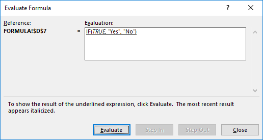
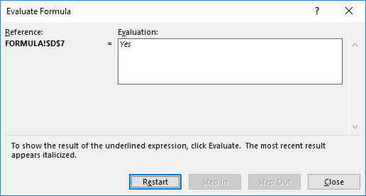
STEP 6:  Since the If formula received a TRUE, Excel evaluated it as a Yes end result. We have seen how the formula gave us the result in a few easy steps!